Reinforcement Learning

Dynamic Programming

(1) Policy iteration: First evaluate current policy by Bellman equation. In particular, compute the state-value function $v_{\pi }$ where $\pi$ denotes the current policy. In any evaluation iteration $k$, the state value at $s$ is updated as:

The the value function for the current policy helps find better policy, namely policy improvement. At any state $s$ we can select a new greedy policy by equation:

The detailed algorithm is presented in the pseudocode below:

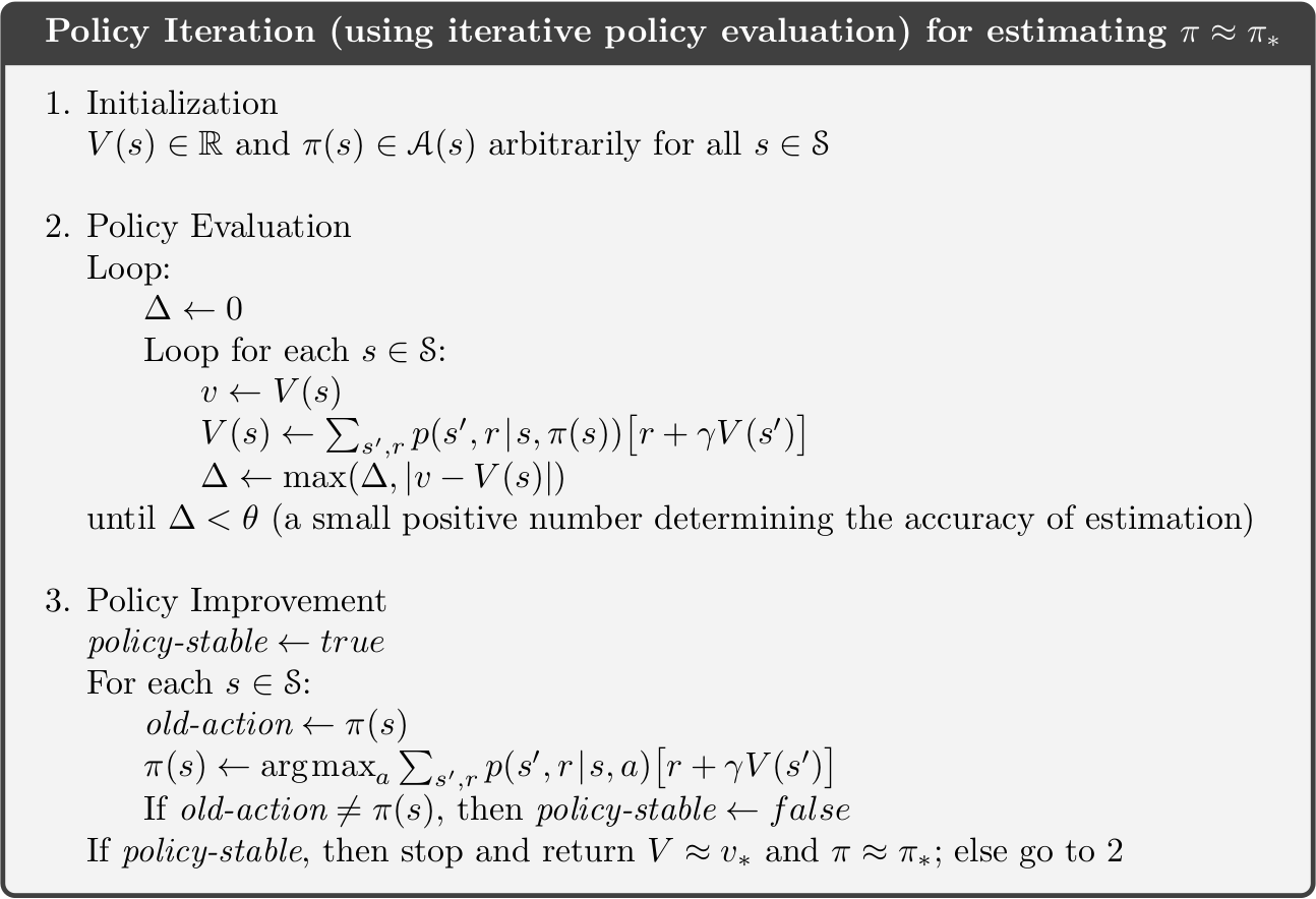
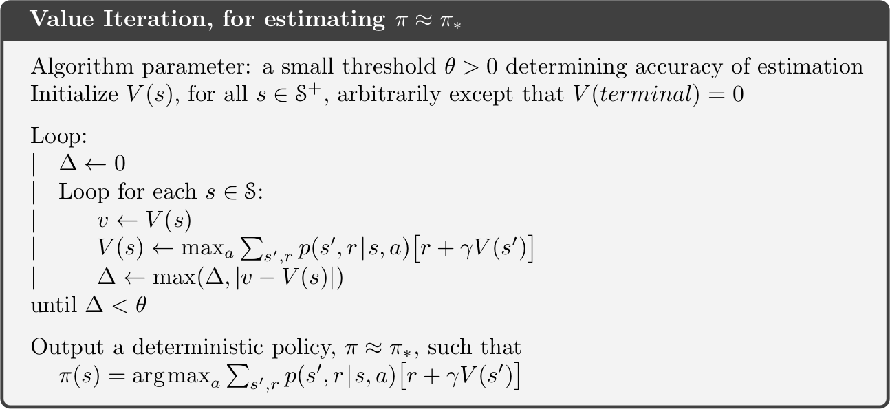
(2) Value iteration: In policy iteration, the policy evaluation involves multiple sweeps through the state set. The policy improvement occurs only when the evaluation converages.

In fact, the policy evaluation can be stopped after just one update of each state. This algorithm is called the value iteration.

Monte Carlo Methods

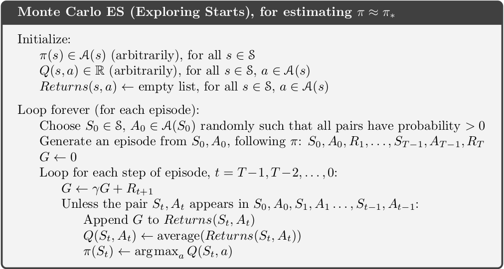
In dynamic programming, it is required that the model of the envrionment’s dynamics is known, which limits its application. The Monte Carlo methods instead learn the value function from experience in the form of sample episodes.

The first MC method is presented here below. One of the greatest difficulties in RL is the fundamental dilemma of exploration versus exploitation: When should the agent try out (perceived) non-optimal actions in order to explore the environment (and potentially improve the model), and when should it exploit the optimal action in order to make useful progress? To maintain sufficient exploration, it is assumed that the episodes have exploring starts and all state-action pairs have probability > 0 to be chosen.

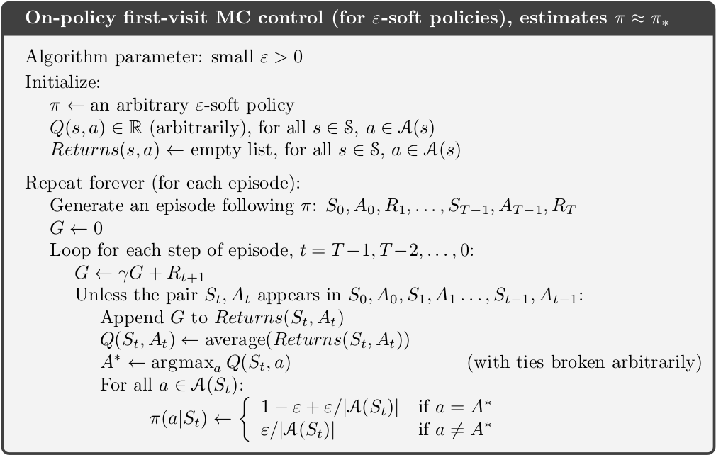
The assumption in the algorithms seems unrealistic. One way to ensure the sufficient exploration is to use a stochastic policy namely $ϵ$-greedy policy such that there is a small chance to select actions that are not evaluated as optimal. The algorithm is presented here.

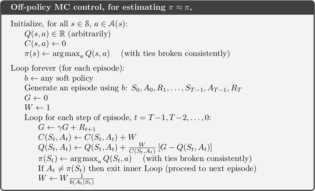
The previous two algorithms are on-policy methods. The off-policy MC control is shown below. The agent follows the behaviour policy while learning about and improving the target policy. Although the target policy may be deterministic, the agent can still sample all possible actions.

Temporal-Difference Learning

TD learning combines ideas of MC methods and DP methods. It does not require model of the envrionment’s dynamic and learns values from the experience, like MC methods. It also updates the estimate based on other estimate and does not have to wait for the return until the episode ends (bootstrapping), like DP methods.

In MC methods, the value of a state is updated as follows $V(S_t)\leftarrow V(S_t)+\alpha [G_t-V(S_t)].$
where $G_t$ is the actual return following time $t$.

In TD methods, agent only needs to wait until the next time step. It updates like this $V(S_t)\leftarrow V(S_t)+\alpha [R_{t+1}+\gamma V(S_{t+1})-V(S_t)].$

Since the agent does not need to wait unitl the episode ends, the TD methods are implementated in an online, fully incremental fashion.

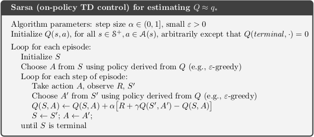
One on-policy TD control method is Sarsa. The target action value is the sum of the immediate reward plus the action value $Q(S^{\prime },A^{\prime })$ where $A^{\prime }$ is chosen by the policy, e.g., $ϵ$-greedy.

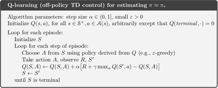
Q-learning is an off-policy TD control method. The action-value function $Q$ is independent of the policy being followed ($ϵ$-greedy). In particular, the target action value is equal to the sum of immediate reward and the maximal action value at successor state $S^{\prime }$. The action $a$ in the target action value is greedy instead of $ϵ$-greedy in Sarsa.

Deep Q-network

Unlike to tabular and traditional non-parametric methods, e.g., Q-learning, Deep Q-network can deal efficiently with the curse of dimensionality. It tries to approximate the action-value function $Q$ based on training deep neural networks.

Reinforcement learning is unstable and even diverge when a nonlinear function approximator such as neural network is used to represent the action-value (Q function). The causes are the correlations present in the sequence of observations. Small updates to Q may significantly change the policy and change the data distribution, and the correlations between action-value (Q) and target value $r+\gamma {\mathrm{m}\mathrm{a}\mathrm{x}}_{a^{\prime }}Q(S^{\prime },a^{\prime })$.

Two key ideas are used to address the correlation:
(1) Replay buffer that randomizes over the data and removes correlation sequence and smoothes over changes in the data distribution.
(2) Update the target value periodically instead of every iteration.

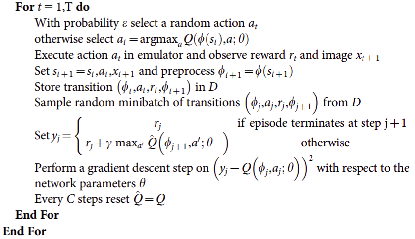
More specifically, the DQN parameterizes an approximate value function $Q(s,a,{\theta }_i)$, where ${\theta }_i$ are the parameters of Q-network at iteration $i$. At each time step $t$, the experience $e_t=(s_t,a_t,r_t,s_{t+1})$ is stored in the replay buffer $D_t=\{e_1,...,e_t\}$. During learning, the experience is drawn randomly from the replay buffer, i.e., $(s,a,r,s^{\prime })\sim U(D)$ and is used to update the parameter by gradient descent. The loss function is:

where ${\theta }_i$ is the parameter of Q-network and ${\theta }_i^{-}$ is the parameter of the target network, which is updated every $C$ steps and held fixed between individual updates. The pseudocode of the algorithm is shown here:

Deep Q learning is (1) model free: not explicitly estimate the reward and transition dynamics. (2) off-policy: learn the greedy policy but execute action based on $ϵ$-greedy behaviour policy for exploration.

Advantage of replay buffer: (1) each step of experience is potentially used in many updates, which allows for greater data efficiency. (2) break the correlation between samples. (3) The behaviour distribution is average over many of its previous states smoothing out learning and aoviding oscillations or divergence in the parameters.

Policy Gradient Methods

The methods introduced above are all categorized as action-value methods, which select the action based on the action-value estimates. Another class of methods consider to learn a parameterized policy that enables actions to be chosen without consulting action-value estimates. Although the action-value function may still be used to learn the policy parameter, e.g., REINFORCE with baseline, but is not required to select the action.

The advantages of policy-based methods are that (1) They can learn appropriate levels of exploration and approach deterministic policies asymptotically. (2) They can learn specific probabilities for taking the actions. (3) They can naturally handle continuous action spaces. (4) The action probabilities change smoothly as a function of learned parameter.

The policy-gradient theorem below gives an exact formula for how performance is affected by the policy parameter which does not depend on the state distribution. This provides a theoretical foundation for all policy gradient methods, which update the policy parameter on each step in the direction of an estimate of the gradient of performance with respect to the policy parameter.

where $\mu (s)$ is the state distribution (on-policy distribution under $\pi$).

REINFORCE: MC Policy Gradient

Now we need to obtain samples such that the expectation of the sample gradient is proprotional to the actual gradient of the performance. This is based on the equations below

$S_t,A_t$ are introduced by replacing a sum over the random variable’s possible values by an expectation under policy $\pi$, then sampling the expectation.

The equation tells us the quantity that can be sampled on each time step whose expectation is equal to the gradient. Therefore the update rule is

where $\alpha$ is the step size, into which the constant of proportionality is absorted.

The updat rule enables the parameter to move most in the directions that favor actions that obtain the highest return. The detailed algorithm is presented below:

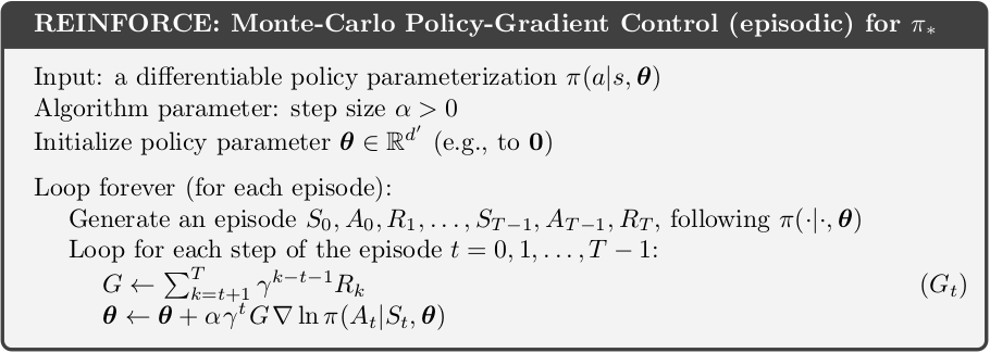
This method is a MC algorithm because the complete return $G_t$ is used (no bootstrapping). However this method may be of high variance and produce slow learning.

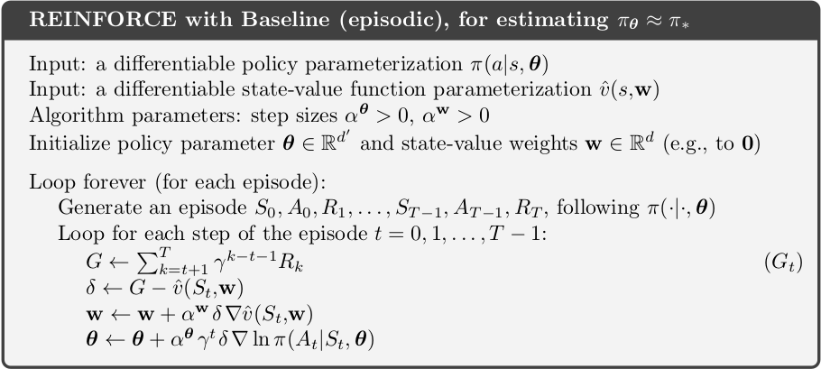
REINFORCE with Baseline

One way to reduce the variance is to include a comparison of the action value to an arbitary baseline $b(s)$, which can be any variable as long as it does not vary with action.

It is intuitive to choose the estimate of the state value, $\hat{v}(S_t,w)$ as the baseline. The value function $\hat{v}(S_t,w)$ can be learned by the gradient descent and $w$ is the state-value parameter. This is the REINFORCE with baseline shown below.

REINFORCE: actor-critic

The previous two methods are unbiased but tend to learn slowly and produce estimates of high variance. Also it is inconvenient to implement online or for continuing problems.

Like TD methods, we can use bootstrapping to replace the full return in target value of REINFORCE with the one-step return. The update rule (with a learned state-value function as baseline) is

Although the bias is introduced through bootstrapping, the variance is reduced substantially and learning thus becomes faster.

The pseudocode is presented below. This is a fully online, incremental algorithm.

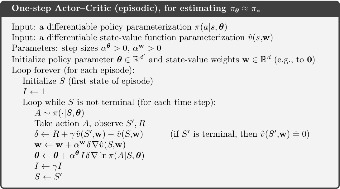
This algorithm is called actor-critic because the state-value function (critic) is used to provide feedback to the policy (actor). Therefore formally, the REINFORCE baseline is not actor-critic because the value function is only used as a baseline, which neither introduces bias nor change the expected value of the update.

Policy-based methods is able to deal with the large actions space, even continuous space with infinite number of actoins. Instead of learning the probability for each individual action, we can learn a probability distributions for each entry of the action (vector), e.g., the mean and variance of the Gaussian distribution.

Deterministic Policy Gradient Algorithms

The methods in previous section is in fact the stochastic policy gradient. The policy is represented by a parametric probability distribution, i.e., ${\pi }_{\theta }:\mathcal{S}\to \mathcal{P}(\mathcal{A})$. However computing the stochastic policy gradient may require more samples, especially if the action space is high-dimentional.

Silver et al. extend the policy gradient theorems for stochastic policies to deterministic, i.e., ${\mu }_{\theta }(s):\mathcal{S}\to \mathcal{A}$. DPG requires fewer samples in problems with high-dimensional action space.

In more details, the general performance objective for the problem is the cumulative (discounted) reward from the start state. For stochastic PG, that is

For deterministic PG, the performance objective is

where ${\rho }^{\pi }(s)$ is the state distribution.

As a result, the performance gradient ${\mathrm{\nabla }}_{\theta }J({\pi }_{\theta })$ for SPG should integrate over both state and action spaces while in DPG it only integrates over the state space.

The paper proposes the deterministic policy gradient theorem as:

Stochastic policy is usually used to explore the full state and action space. To ensure the sufficient exploration, an off-policy actor-critic algorithm is derived based on the theorem. Specifically, the agent takes actions based on a stochastic behaviour policy $\beta (s|a)$ and learns a deterministic target policy ${\mu }_{\theta }(s)$. The action-value function $Q^w(s,a)$ (critic) approximates the true function $Q^{\mu }(s,a)$. The basic structure is similar to the REINFORCE actor-crtic. The parameter for actor $\theta$ and critic $w$ are updated as following

Deep Deterministic Policy Gradient Algorithms

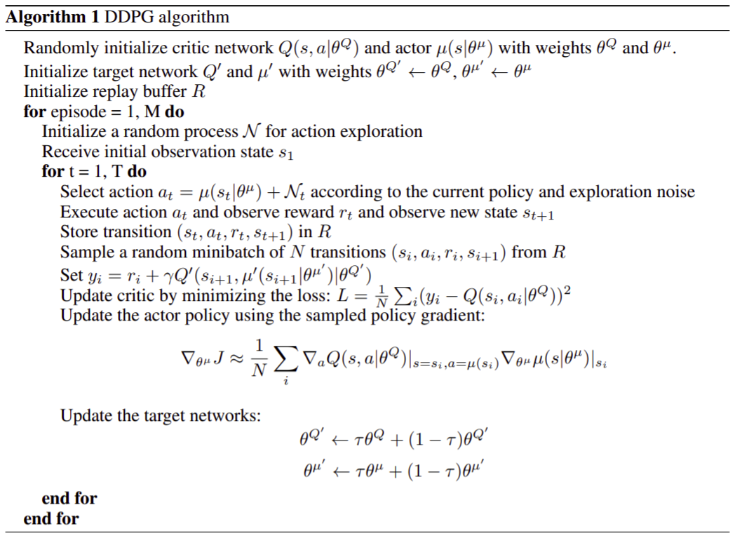
The paper introduces Deep Deterministic Policy Gradient Algorithms that combine the idea of DQN and DPG, and can learn policies in high-dimensional, continuous action spaces.

Similar to DQN, a replay buffer is used to address the correlation in the sequence of observations. The transition $(s_t,a_t,r_t,s_{t+1})$ sampled based on the behaviour policy is stored in the replay buffer. In each time step, a minibatch is uniformly taken from the replay buffer and is used to update the actor and critic.

DDPG uses soft target updates, instead of directly copying the weights in DQN. The weights of the target networks ${\theta }^{\prime }$ are updated by make them slowly track the learned network: ${\theta }^{\prime }\leftarrow \tau \theta +(1-\tau ){\theta }^{\prime }$ with $\tau \ll 1$. Consequently the target values change slowly, which improves the stability of learning.

DDPG is off-policy. The behaviour policy and actor policy should be different. A noise process $\mathcal{N}$ is added, i.e.,

The pseudocode is presented below:

To be continued …

Terminology

on-policy methods: The agent commits to always exploring and tries to find the best policy that still explores.

off-policy methods: The agent also explores, but learns a deterministic optimal policy that may be unrelated to the policy followed. It is usually based on some form of importance sampling, i.e., on weighting returns by the ratio of the probabilities of taking the observed actions under the two policies, thereby transforming their expectations from the behavior policy to the target policy.

action-value methods: learn the value of actions and select actions based on the estimated action values, e.g., Q-learning, TD learning.

Bootstrapping: Update estimate of state value (action value) based on the estimate of state value (action value) of the successor state.

actor-critic: methods that learn approximations to both policy and value functions. The actor refers to the learned policy and critic refers to the learned value function.