Full SLAM with FastSLAM Algorithm
The FastSLAM algorithm implemented in this project solves the full SLAM problem. It uses particle filters for estimating the robot path while each particle (which is a hypothesis of robot pose) uses separate EKFs to estimate each map feature location, based on the conditional independence between any two disjoint sets of features in the map, given the robot pose. The particle in FastSLAM is denoted as
\[\langle x_t^{[k]}, \mu_{1,t}^{[k]}, \Sigma_{1,t}^{[k]}, ..., \mu_{N,t}^{[k]}, \Sigma_{N,t}^{[k]} \rangle\]where \(k\) is the index of the particle, \(\mu_{i,t}^{[k]}, \Sigma_{i,t}^{[k]}\) refer to the mean and covariance of the i-th map feature.
The advantage of FastSLAM is
-
The data association decision can be made on a per-particle basis. The FastSLAM maintains multiple data associations, in contrast to EKF that tracks only one at any time step
-
The particle filter used in FastSLAM allows the algorithm to deal with the highly nonlinear motion models.

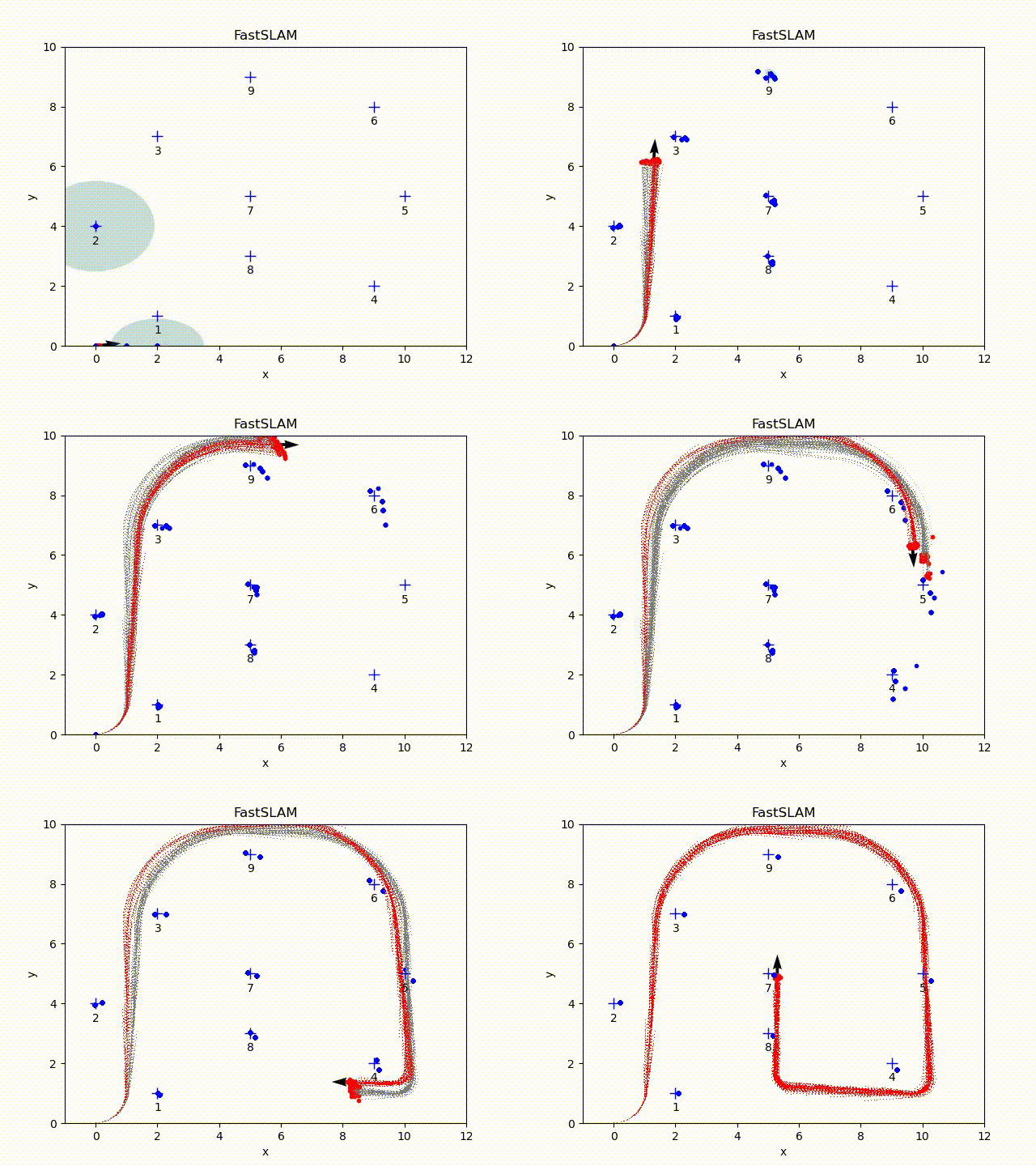
The particles with the highest weight are in red color. The arrow refers to the current pose of the particle with the highest weight. All other particles are in gray color (some of paths may be disappear because of the resampling step). The blue crosses represent the ground-true position of the landmarks. The blue dots represent the estimated landmark positions of each particle. The ellipse is the error ellipse of estimated landmark positions of the particle with the highest weight.
FastSLAM Overview
The full SLAM problem considered in this project can be written as a posterior:
\(P(x_{0:t},m_{1:N}|z_{1:t},u_{1:t}) = P(x_{0:t}|z_{1:t},u_{1:t}) P(m_{1:N}|x_{0:t},z_{1:t})\).
Based on the conditionally independence of the landmarks given the poses, the latter posterior on the right hand side can be further written as
\[\prod*{i=1}^{N} P(m_i|x*{0:t},z\_{1:t})\]Therefore the full SLAM posterior is equivalent to:
\[P(x*{0:t},m*{1:N}|z*{1:t},u*{1:t}) = P(x*{0:t}|z*{1:t},u*{1:t})\prod*{i=1}^{N} P(m*i|x*{0:t},z\_{1:t})\]The path posterior can be represented by a set of the particles while each particle maintains separate map posterior by EKF, i.e.,
\[\langle x*t^{[k]}, \mu*{1,t}^{[k]}, \Sigma*{1,t}^{[k]}, ..., \mu*{N,t}^{[k]}, \Sigma\_{N,t}^{[k]} \rangle\]The key steps of FastSLAM are following:
- Prediction: Extend the path posterior by sampling a new pose for each particle, based on the motion model (odometry motion model in this project).
-
Measurement update: Update belief of each observed landmark by EKF, compute measurement predication by
\[\hat{z}^{[k]} = h(\mu^{[k]}_{j,t-1}, x_t^{[k]})\] -
Compute the particle weight by
\[w^{[k]} = |2\pi Q|^{-\frac{1}{2}} \exp{(-\frac{1}{2}(z_t - \hat{z}^{[k]})^T Q^{-1} (z_t-\hat{z}^{[k]}))}\]
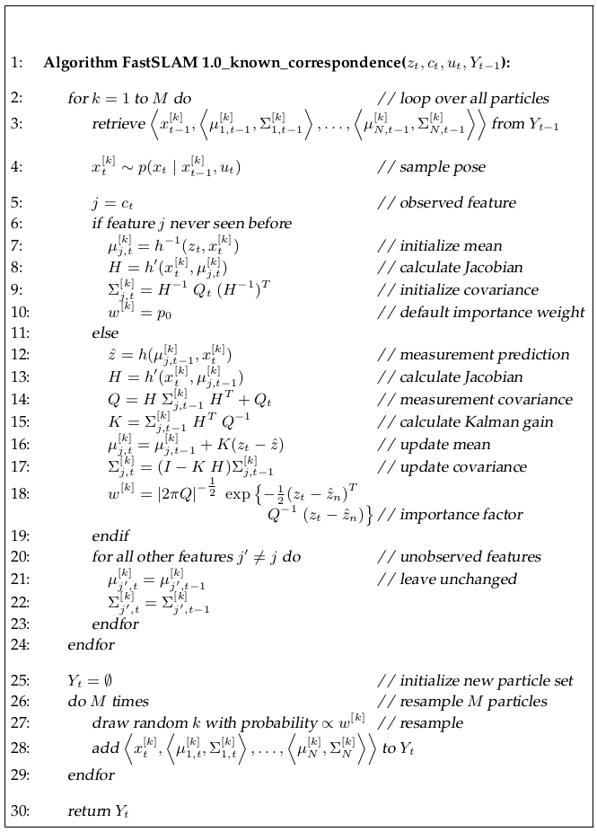
The detailed algorithm is presented in the pseudocode[2] below.

Code Explanation
-
sample_motion_model(odometry, particles): Sample a new pose for each particle by the odometry motion model. Implement line 3 to 4. -
measurement_model(particle, landmark): Compute the expected measurement for the given landmark and the Jacobian with respect to the landmark. Implement line 12 to 13. -
eval_sensor_model(sensor_data, particles): Update the estimate of the landmark position based on the range-bearing measurement[1] and compute the particle weight.
Repository
References
-
Introduction to Mobile Robotics
University of Freiburg, Spring, 2020, http://ais.informatik.uni-freiburg.de/teaching/ss20/robotics/index_en.php -
Probabilistic Robotics
S. Thrun, W. Burgard, and D. Fox. MIT Press, Cambridge, Mass., (2005)