Online SLAM with Unscented Kalman Filter
Generally speaking, the Kalman filters require linear motion model and sensor model to perform the transformation of Gaussian distribution. In EKF, the first order Taylor expansion is used to linearize the functions at the mean of the belief. An alternative linearization method, called unscented transform is used in the Unscented Kalman Filter. In particular, the UKF extracts a set of points with weights from the Gaussian and passes those points through the nonlinear function. The transformed Gaussian can be recovered from those returned points.
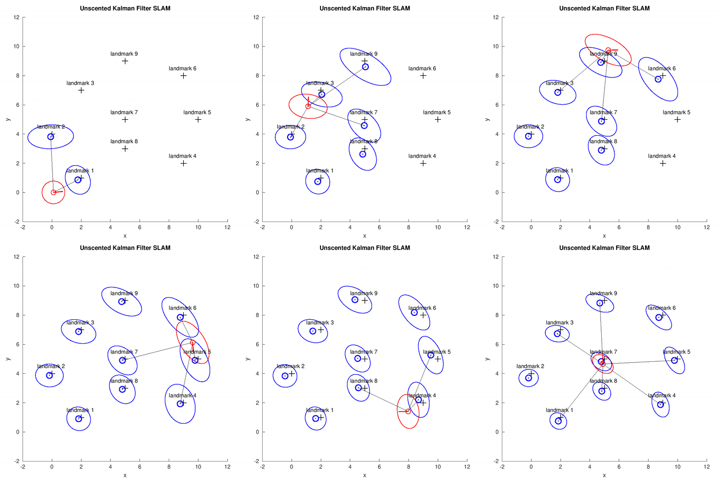
In this project, we implemented a UKF for the online SLAM problem. Similar to the EKF, given the sensor reading, odometry information and the data association[1], the robot estimates the its pose (shown by the red covariance ellipse and bar), the position of map feastures (shown by the blue covariance ellipse) at each time step.

UKF Overview
The points extracted from a Gaussian is called the sigma points, denoted by \(\chi^{[i]}\) and weight \(w_m^{[i]}\) and \(w_c^{[i]}\). For a \(n\)-dimensional Gaussian with mean \(\mu\) and covariance \(\Sigma\), the sigma points are computed according to:
\[\begin{equation*} \begin{split} \chi^{[0]} &= \mu \\ \chi^{[i]} &= \mu + (\sqrt{(n+\lambda)\Sigma})_i, \ &\forall i = 1, ..., n \\ \chi^{[i]} &= \mu - (\sqrt{(n+\lambda)\Sigma})_{i-n}, \ &\forall i = n+1, ..., 2n \\ \end{split} \end{equation*}\]where subscript \(i\) denotes the index of the column and \(\lambda\) is a scaling parameter.
The two weights for each sigma point is computed by:
\[\begin{equation*} \begin{split} w^{[0]}_m &= \frac{\lambda}{n+\lambda} \\ w^{[0]}_c &= \frac{\lambda}{n+\lambda} + (1-\alpha^2+\beta) \\ w^{[i]}_m &= w^{[i]}_c = \frac{1}{2(n+\lambda)}, \ \forall i = 1, ..., 2n. \end{split} \end{equation*}\]where \(w^{[i]}_m\) is used to recover the mean \(\mu\) while \(w^{[i]}_c\) is used to recover the covariance \(\Sigma\).
The the sigma points are passed to the nonlinear function say \(g(x)\), i.e.,
\[\mathcal{Y}^{[i]} = g(\chi^{[i]})\]The transformed Gaussian distribution can be recovered from the returned sigma points \(\mathcal{Y}^{[i]}\).
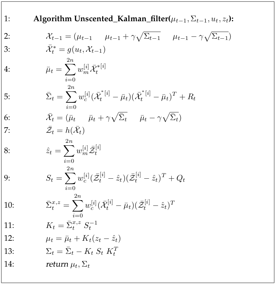
\[\begin{equation*} \begin{split} \mu' &= \sum_{i=1}^{2n} w_m^{[i]} \mathcal{Y}^{[i]} \\ \Sigma' &=\sum_{i=1}^{2n} w_c^{[i]}(\mathcal{Y}^{[i]} - \mu') (\mathcal{Y}^{[i]} - \mu')^T \end{split} \end{equation*}\]Using the transformation mentioned above, the predication step in EKF can be replaced by the sigma point propagation of the motion model. Similarily in correction step we can pass the obtained sigma points (of the predicted Gaussian) to the sensor model \(h(x)\), and recover the mean and covariance of the expected observation. The Kalman gain then can be computed from the covariance of the observation and the cross-covariance between state and observation. The detailed algorithm[2] is shown below:

Note that \(S_t\) in line 9 is equivalent to \(H_t \bar{\Sigma}_t H_t^T + Q_t\) and \(\bar{\Sigma}_t^{x,z}\) in line 10 is equivalent to \(\bar{\Sigma}_t H_t^T\) in computing the Kalman gain in EKF, i.e., \(K_t = \bar{\Sigma}_t H_t^T (H_t \bar{\Sigma}_t H_t^T + Q_t)^{-1}\)
Code Explanation
-
[mu, sigma, sigma_points] = prediction_step(mu, sigma, u): implement line 2 to 6 of the algorithm above, compute the mean and covariance of the state which includes the robot’s pose and landmark positions. -
[mu, sigma, map] = correction_step(mu, sigma, z, map): implement the correction step from line 7 to 13 in UKF algorithm, update the mean and covariance of state after the range-bearing sensor measurement.
Repository
References
-
Robot Mapping
University of Freiburg, WS 2013/14, http://ais.informatik.uni-freiburg.de/teaching/ws13/mapping/ -
Probabilistic Robotics
S. Thrun, W. Burgard, and D. Fox. MIT Press, Cambridge, Mass., (2005)