Bag of Visual Word for Finding Similar Images
A key problem for range-bearing sensors is known as the data association problem, which arises when landmarks cannot be uniquely identified. Therefore some residual uncertainty exists with regards to the identity of a landmark. A similar problem happens in the graph construction of the GraphSLAM (see more details in here). We need to match the observation to obtain the constraint. The problem arises when only the range-bearing sensor is used. For example, the robot may not distinguish the laser range data for the corridors because the corridors may look exactly the same from a laser sensor.
To obtain the addition information of the map features, we can use camera to take the images of the environment and comparing those images to distinguish the map features. For example, we can write numbers on walls of different corridors. The robot can tell if the observed corridor is the same one observed before by comparing the images.
In this project, a C++ application is created to compare images. Given a database of images and a query image, the program is able to find to N most similar database image to the query image.
Overview of Bag of Visual Words
The basic idea comes from the “bag of words” which is originally used for comparing text documents. More specifically, similar papers can be found by first counting the occurrences of certain words and then return documents with similar counts.
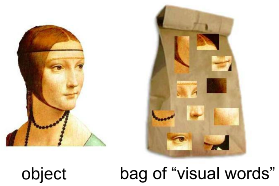
Similar idea can be applied to the images. We can treat the independent features in an image as the visual words and construct a visual dictionary of the representative words, as shown in figure below[1]. Then quantize features of image using visual dictionary. Each image can be represented by a histogram of visual word occurrences. Image comparisons are performed based on such word histograms.

To construct the dictionary, we first need to extract feature descriptors (SIFT is used in this project) from the given training dataset. Each feature descriptor can be treated as a point in high-dimentional space. All feature descriptors are then grouped into different sets by the k-meaning clustering. More specifically, the points are partitioned into k clusters which are represented by the mean of points in the cluster, i.e., centroids. The basic procedure of k-mean clustering is following
- Choose k arbitrary centroids as cluster representatives
- Assign each data point to the closest centroid.
- Re-compute the centroids of the clusters based on the assigned data points.
- Go back to step 2 until convergence.
Now each centroid obtained by k-mean clustering is one visual word in the dictionary. All images can be represented by a set of visual words and a histogram of the word occurrences can be further obtained. The histogram is a compact summary of the image content whith several nice properties. It is largely invariant to the viewpoint changes and deformations. Also it ignores the spatial arrangement.
The next question is to how to find similar images by comparing the word occurrence histograms of images. First we weight words based on the probability that they appear. The weight is computed by TF-IDF shown in equation below.
\[t_{id} = \frac{n_{id}}{n_d} \log{\frac{N}{n_i}}\]where \(n_{id}\) refers to the occurances of word \(i\) in image \(d\), \(n_d\) refers to the number of all word occurences in image \(d\), \(n_i\) denotes the number of images containing word \(i\), and \(N\) denotes the number of the images in the training set.
The histogram can be reweighted by replacing the word occurences with the obtained \(t_{id}\). As a result, the relevant visual words get higher weights while words that occur in every image are weighted down to zero. Now the reweighted histograms can be compared by computing the angle between the two vectors in which each entry is equal to the \(t_{id}\) value for each bin of the histogram. In particular, we compute the cosine distance between two vectors, i.e.,
\[1 - \frac{x^T y}{\|x\| \|y\|}\]The cosine distance varies from \(0\) to \(1\).
To sum up, the procedure of the image finder in this project is following:
- Create a dictionary that contains visual words obtained by extracting SIFT feature descriptors from the training set images and k-mean clustering.
- Create a database that stores TF-IDF weighted histograms for all database images.
- Extract SIFT feature descriptors from the qeury image and assign them to visual words in the dictionary.
- Build TF-IDF histogram for the query image.
- Return N most similar images by computing the cosine distance of histograms between the query image and dataset image.
Note that computing SIFT descriptors is time consuming. In this project, the SIFT descriptors is computed and coverted into a binary file. In this way, we don’t have to compute SIFT every time a comparison is needed and it is easier to update the dataset images. We also store the TF-IDF weighted histograms of dataset images into a .csv file for the same reason.
Compiling instruction
This project uses OpenCV 4 library for extracting SIFT features and k-mean clustering. The dataset is provided at Page 69 in the slides.
To compile the code, type following commands at the root directory of the project.
mkdir build
cd build
cmake ..
make
There are four executables created in results/bin. More specifically,
-
create_data_bin: compute SIFT descriptors for all dataset image and serialize the data into a binary file. -
create_distionary: construct the dictionary of the visual words. -
create_histograms: compute the TF-IDF histograms of dataset images and store the corresponding vectors intoReweighted_histogram.csvfile. -
find_similar_imgs: compute the SIFT feature descriptors of the query image and TF-IDF histogram. Compute the cosine distance between the vector of query image and dataset images inReweighted_histogram.csvfile. Create a html file that contains N most similar images in the dataset.
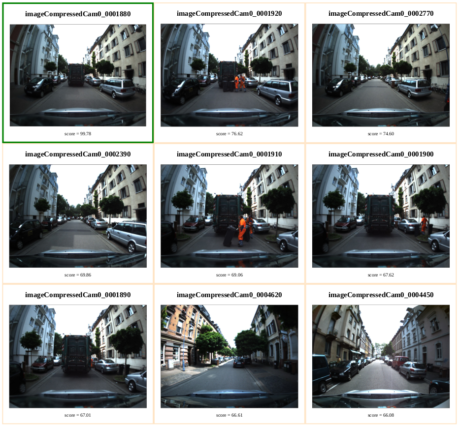
Given the query image imageCompressedCam0_0001880, the program finds following most similar images in the dataset.

The most similar image shown here is in fact the query image. You can also see the created hmtl page here.
Repository
References
-
CS131 Computer Vision: Foundations and Applications
Stanford University, Fall 2017, http://vision.stanford.edu/teaching/cs131_fall1718/ -
Modern C++ Course For CV
University of Bonn, 2020, https://www.ipb.uni-bonn.de/html/teaching/modern-cpp/slides/bow.pdf