IMU Preintegration based Lidar Inertial Odometry

This project implements a tightly coupled 3D lidar inertial odometry based on IMU preintegration. Given 3D lidar scan and IMU sensor data, the goal is to create 3D point cloud map of the environment. The state estimation is achieved by pose graph optimization with both imu preintegration measurement and point cloud alignment involved as residuals. The optimization problem is built for estimating the state of two consecutive frames, though it can be further adapted to integrate more frames and observations by modifying objective function. Moreover the marginalization is implemented and executed for smoothing the state estimation.

Key Components

1. IMU preintegrator
2. Incremental NDT matcher
3. Pose graph optimization
4. Lidar-inertial odometry
5. Data synchronization

IMU preintegrator

Goal: Compute IMU preintegration measurements, i.e., rotation, velocity, position: $\Delta \tilde{R}_{ij}, \Delta \tilde{v}_{ij}, \Delta \tilde{p}_{ij}$. Compute covariance of preintegration measurement noise. Compute Jacobian of bias for bias update. Predict current IMU state, given state at a start point.

Procedures

1. Update preintegration measurement $\Delta \tilde{R}_{ij}, \Delta \tilde{v}_{ij}, \Delta \tilde{p}_{ij}$ based on received IMU readings.
2. Update covariance of measurement noise, i.e., $\Sigma_{ij} \in \mathbb{R}^{9 \times 9}$ based on covariance at previous timestep $\Sigma_{i j-1}$ and covariance of IMU sensor $\Sigma_{\eta} \in \mathbb{R}^{6 \times 6}$.
3. Update Jacobian for bias update. The Jacobian describes how the measurement change due to a change in bias estimate. All updates are computed incrementally.
4. IMU preintegration measurements are used for creating pose graph optimization problem in which the residuals are defined as difference between measurement and measurement model.
   • $r_{\Delta R_{ij}} = \mathrm{Log}(\Delta \tilde{R}_{ij}^T R^T_i R_j)$
   • $r_{\Delta v_{ij}} = R^T_i (v_j - v_i - g \Delta t_{ij}) - \Delta \tilde{v}_{ij}$
   • $r_{\Delta p_{ij}} = R^T_i (p_j - p_i - v_i \Delta t_{ij} - 0.5 g \Delta t_{ij}^2) - \Delta \tilde{p}_{ij}$
5. The measurements are also used to compute the Jacobian of residual errors for solving optimization problem at each Gauss-Newton iteration.
6. Reset measurements to 0, after pose graph optimization is solved.

Code

• source code

Incremental NDT matcher

Goal: estimate the current global pose by NDT alignment of source and target point cloud. The statistics of NDT target grid cell is updated incrementally.

Procedure

1. Given the initial target point cloud, grid resolution (voxel cell size), align each scan point to a voxel cell and compute the mean and variance of scan point positions for each voxel cell.
2. Align source point cloud to target point cloud by solving least square problem. The residual is the sum of the difference between the transformed source scan point and target point, i.e., $\sum_i \left \lVert R * p_{si} + t - p_{ti} \right \rVert_{\Sigma_i}$
3. The solution is used as a SE(3) observation in the pose graph optimization.
4. If current frame is determined as a keyframe, add source point cloud to NDT matcher and update target grid statistics incrementally. See more detailed description in LIO3D.

Code

• source code

Pose Graph Optimization

Goal: Build pose graph optimizaton with g2o. Estimate current states such that the residuals is minimized. The states are position, velocity, rotation, bias of gyroscope, accelerometer, and gravity. The residuals include imu preintegration residuals described above, prior factor, bias factors, NDT alignment.

Procedures

1. Define the vertices, namely the states at the beginning and end of imu preintegration, i.e., $p_i, p_j, v_i, v_j, \phi_i, \phi_j, b_{gi}, b_{gj}, b_{ai}, b_{aj}$.

2. Define edges:

   • preintegration factors: $[\mathbf{r}^T_{\Delta R_{ij}}, \ \mathbf{r}^T_{\Delta v_{ij}}, \ \mathbf{r}^T_{\Delta p_{ij}}]^T$, jacobian see reference[1]. The information matrix is computed from the covariance of measurement noise. To reduce the impact of outliers, the Huber robust kernel is used.
   • prior factors: $[\mathrm{Log}(R_{i,prior}^T R_i)^T, \ (p_i - p_{i, prior})^T, (v_i - v_{i, prior})^T, \ (b_{ai} - b_{ai, prior})^T, \ (b_{gi} - b_{gi, prior})^T ]^T$. $\mathrm{Jacobian} = \mathrm{diag}(J_r^{-1}(R_{i,prior}^T R_i), \mathbf{I}_3, \mathbf{I}_3, \mathbf{I}_3, \mathbf{I}_3)$ The information matrix is computed by marginalization of the Hessian matrix from the last optimization.

   • NDT alignment: $[\mathrm{Log}(R_{j,ndt}^T R_j)^T, (p_j - p_{j, ndt})^T]^T$ $\mathrm{Jacobian} = \mathrm{diag}(J_r^{-1}(R_{i,gnss}^T R_j), \ \mathbf{I}_3)$

   • Gyroscope Bias factor: $b_{g, j} - b_{g, i}$, jacobian = $[-\mathbf{I}_3, \mathbf{I}_3]$
   • Accelerometer Bias factor: $b_{a, j} - b_{a, i}$, jacobian = $[-\mathbf{I}_3, \mathbf{I}_3]$

3. Solve optimization problem. Asign optimizaed states to current states.

4. Compute the information matrix of the prior factor for the next optimization by marginalizing the vertices at time step i.

   • Compute the approximate Hessian matrix $H = J^T \Sigma^{-1} J \in \mathbb{R}^{30 \times 30}$ where \(J_i = \begin{bmatrix}A &B \\B^T &C \end{bmatrix}\)

   • The matrices $A, B \in \mathbb{R}^{15 \times 15}$ are the components of Hessian related to state at time step i.
   • Eliminate first 15 rows and cols by Schur complement, i.e. $\tilde{C} = C - B^T A^+ B \in \mathbb{R}^{15 \times 15}$, where $A^+$ denote the pseudo inverse of $A$
   • Matrix $\tilde{C}$ is used as the information matrix of prior factor for the next optimization problem.

Code

• Definition of vertices and edges
• Building pose graph and marginalization

Lidar-inertial odometry

Goal: Estimate the states at each time step given synchronized lidar and imu data. The states are estimated by pose graph optimization.

Procedure

1. Initialize IMU by integrating gyroscope and accelerometer readings while the robot keeps static. Compute bias and covariance of gyroscope and accelerometer noise, gravity, which are used in IMU preintegration.

2. Add imu reading to IMU preintegrator and update imu preintegration measurment and covariance of noises incrementally.

3. Undistort lidar scan influenced by motion. The undistortion computes the global pose of lidar sensor when scan point is observed ($T_{WLi}$) by interoplating imu poses, and then transform scan point to the last imu reading ($p_{Le}$). More precise $p_{Le} = T_{LI} * T_{IeW} * T_{WIi} * T_{IL} * p_{Li}$

4. Estimate current pose by NDT alignment. The initial guess is predicted from IMU preintegrator.

5. Build and solve pose graph optimization. The residuals include the prior factor of the last frame states, imu preintegration measurement, bias factors, NDT alignment used as a SE(3) observation. The pose of current frame is corrected from the optimized states.

6. Marginalize states of last frame, compute information matrix for the prior factor used in the next optimization. Reset IMU preintegrator.

7. Create keyframe if the motion relative to the last keyframe is over the threshold. Add source point cloud to NDT matcher incrementally.

Code

• source code

• unit test: ./test/preint_test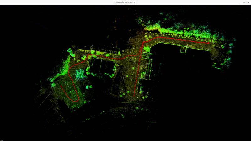

  
  IMU preintegration based lidar-inertial odometry
  
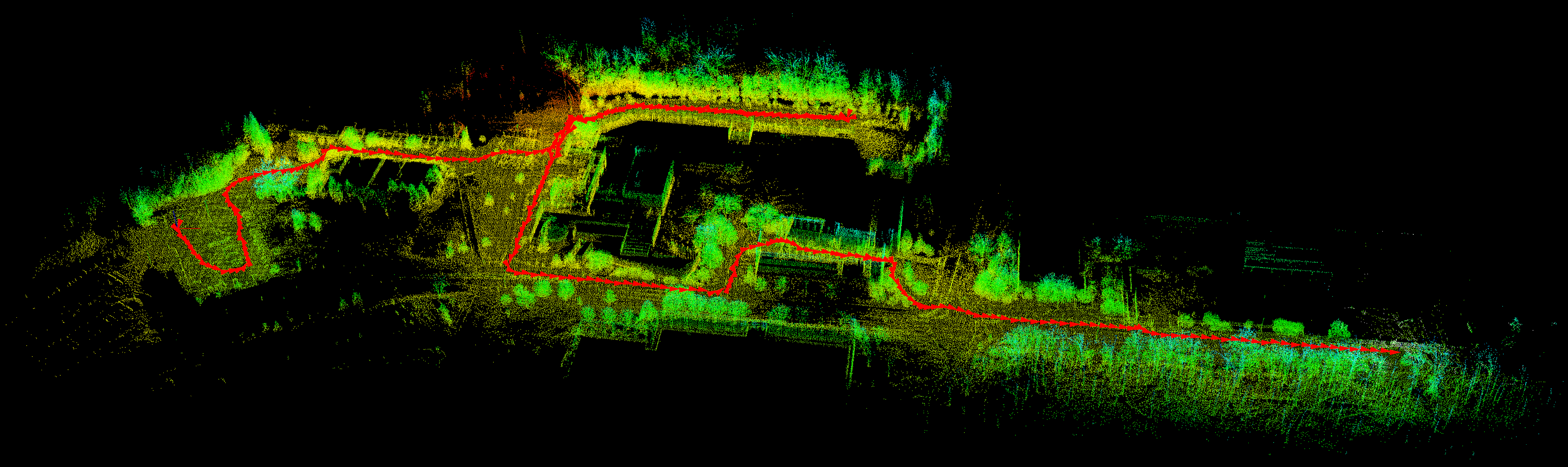  3D point cloud map

Data synchronization

Goal: Match point cloud data with imu readings such that the lidar points from an entire scan is covered imu readings. The motion of the lidar sensor during the scan can therefore be estimated by interpolating the nearest pair of imu readings.

1. put incomming imu and lidar data to deques.

2. create a data group, comprised of one lidar scan and imu readings covering the elapsed time of that scan. In other words, the data group takes from deque all imu readings with timestamp between the start time and end time of the scan.

3. transfer the data group to LIO by callback function.

Code

• source code

Repository