Extended Kalman Filter for Localization

The Kalman filter is a technique for filtering and prediction in linear Gaussian systems. It is assumed that

1. The initial belief \(bel(x_0)\) is normally distributed.

2. The motion model \(P(x_t|x_{t-1}, u_t)\) is a linear function with additional Gaussian noise, i.e.,

   \[\begin{equation}\label{motion} x_t = A_t x_{t-1} + B_t u_t + \epsilon_t \end{equation}\]

3. The observation model \(P(z_t|x_t)\) is linear with Gaussian noise.

   \[\begin{equation}\label{observation} z_t = C_t x_{t} + \delta_t \end{equation}\]

These assumptions are crucial for the correctness of the KF. The efficiency of KF is due to the fact that any linear transformation of a Gaussian random variable results in another Gussian random variable which can be computed in closed form.

However, in most robotics system, the motion model and observation model are nonlinear. To deal with the nonlinearity, the Extended Kalman Filter linearizes the nonlinear function by the first order Taylor expansion and computes a Gussian approximation to the true belief.

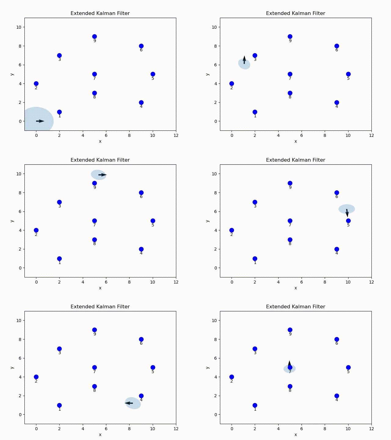
In this project, I implemented the EKF in Python. Given the ground-true position of the landmark, sensor readings and odometry data^[1], at each time step the robot estimate the current pose parameterized by mean and covariance of a Gaussian distribution. The belief is visualized by the arrow indicating the mean pose and covariance ellipse.

EKF Overview

The extended Kalman Filter relaxes one of the assumptions, the linearity assumption. More specifically, the matrix \(A_t\), \(B_t\) in motion model Eq.\(~\eqref{motion}\) and \(C_t\) in observation model Eq.\(~\eqref{observation}\) are now replaced by nonlinear function \(g\) and \(h\).

The nonlinear functions are approximated by linear functions using first-order Taylor explansion, i.e.,

where \(\mu_{t-1}\) is the mean of the posterior of previous time step \(x_{t-1}\). Let \(G_t := \frac{\partial g(u_t, x_{t-1})}{x_{t-1}}|_{x_{t-1}=\mu_{t-1}}\), which is the Jacobian matrix.

Similar to the observation model:

where \(\bar{\mu}_t\) is the mean of the predicted posterior and \(H_t\) is the Jacobian of \(h(x_t)\) with respect to \(x_t\) at \(\bar{\mu}_{t}\), i.e.,

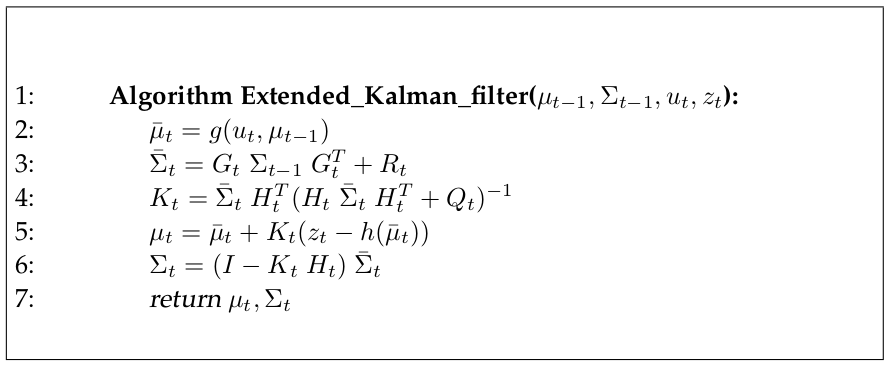
The EKF basically replace the linear prediction by the nonlinear generalizations in EKF. In particular, the linear system matrices \(A_t\) and \(B_t\) are replaced by \(G_t\) and \(C_t\) is replaced by \(H_t\). The detailed algorithm^[2] is presented below.

Code Explanation

1. prediction_step(odometry, mu, sigma): given the odometry and the estimate of the previous pose, motion noise, return the predicted pose in the current time step using the Jacobian of the noise-free odometry motion model.

   \[G_t = \begin{bmatrix} 1 & 0 & -\delta_{tran} \sin(\mu_{\theta_{t-1}}+\delta_{rot1}) \\ 0 & 1 & \delta_{tran} \cos(\mu_{\theta_{t-1}}+\delta_{rot1}) \\ 0 & 0 & 1 \end{bmatrix}\]

   where \(\mu_{\theta_{t-1}}\) is the mean of the estimated orientation of the previous time step.

2. correction_step(sensor_data, mu, sigma, landmarks): given the sensor readings, the ground-truth position of the landmarks and the predicated pose of current time step, return the corrected pose using Jacobian \(H_t\).

   \[H_t = \begin{bmatrix} \frac{\mu_{x_t} - \ell_x^{(k)}}{f(\mu_t, \ell^{(1)})} & \frac{\mu_{y_t} - \ell_y^{(1)}}{f(\mu_t, \ell^{(1)})} & 0 \\ \frac{\mu_{x_t} - \ell_x^{(k)}}{f(\mu_t, \ell^{(2)})} & \frac{\mu_{y_t} - \ell_y^{(2)}}{f(\mu_t, \ell^{(2)})} & 0 \\ \vdots & \vdots & \vdots \\ \frac{\mu_{x_t} - \ell_x^{(k)}}{f(\mu_t, \ell^{(k)})} & \frac{\mu_{y_t} - \ell_y^{(k)}}{f(\mu_t, \ell^{(k)})} & 0 \\ \end{bmatrix}\]

   where \(k\) is number of the sensors, \(\ell^{(i)} = (\ell_x^{(i)}, \ell_y^{(i)})^{T}\) is the position of the landmark, \(\mu_t = (\mu_{x_t}, \mu_{y_t}, \mu_{\theta_t})^T\) is the mean of the predicated pose \(\bar{x}_t\) obtained from the prediction step. Further \(f(\mu_t, \ell^{(i)})\) returns the expected distance to the landmark \(i\)

   \[f(\mu_t, \ell^{(i)}) = \sqrt{(\mu_{x_t} - \ell_x^{(i)})^2 + (\mu_{y_t} - \ell_y^{(i)})^2}\]

References

1. Introduction to Mobile Robotics
   University of Freiburg, Spring, 2020, http://ais.informatik.uni-freiburg.de/teaching/ss20/robotics/index_en.php

2. Probabilistic Robotics
   S. Thrun, W. Burgard, and D. Fox. MIT Press, Cambridge, Mass., (2005)