Occupancy Grid Map
Map is a crucial part of the autonomous robot system. Many applications like localization, path planning and navigation rely on the map. In this project, the occupancy grid mapping algorithm is impelmented to construct a map with assumption that the robot’s poses are known. In occupancy grid map, the space is discretized into independent cells and each cell associates a binary variable estimating if the cell is occupied. More specifically given the sensor readings and robot’s poses in each time step[1], the algorithm computes the log odds of the posterior for each grid \(P(m_i|z_{1:t},x_{1:})\). The occupied grid is black; the free grid is white; the unknow grid is gray. The green dots refer to the robot’s poses. The red dots refer to the end point of the laser scan.
Overview of Occupancy Grid Mapping Algorithm
Grid map is a popular model for representing the environment. The basic idea is to discretize the space into independent cells. Each cell associates to a binary random variable estimating whether the cell is occupied.
The occupancy grid mapping algorithm implement approximate posterior estimation for those random variables. Let \(m_i\) denotes the grid cell, the posterior is \(p(m_i|z_{1:t}, x_{1:t})\).
The log odds ratio \(l(x)=\log \frac{p(x)}{1-p(x)}\) is used to prevent the numerical instabilities for probabilities near zeros or one. It is easy to recover the probability by \(p(x) = 1 - \frac{1}{1+\exp l(x)}\)
We can derive the following relation of posterior.
\[\begin{equation}\label{posterior} l(m_i|z_{1:t}, x_{1:t}) = l(m_i|z_t,x_t) + l(m_i|z_{1:t-1}, x_{1:t-1}) - l(m_i) \end{equation}\]where \(l(m_i|z_t,x_t)\) is called inverse sensor model, \(l_0:=l(m_i)\) is the prior of occupancy.
Let \(l_{t,i} := l(m_i|z_{1:t},x_{1:t})\), based on relation in Eq.\(~\eqref{posterior}\) the occupancy grid mapping algorithm[2] is following.
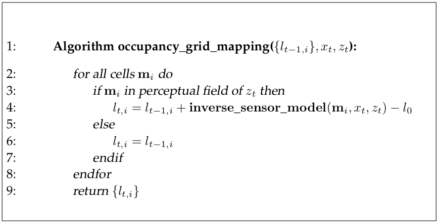
Code Explanation
-
l=prob_to_log_odds(p)converts probability valuepto the corresponding log oddsl.p = log_odds_to_prob(l)converts log oddslto the corresponding probability valuep. -
[pntsMap] = world_to_map_coordinates(pntsWorld, gridSize, offset)converts points from the world coordinates frame to the corresponding coordinates in the grid map frame. -
[mapUpdate, robPoseMapFrame, laserEndPntsMapFrame] = inv_sensor_model(map, scan, robPose, gridSize, offset, probOcc, probFree)computes the log odds values that should be added to the map based on the inverse sensor model of a laser range finder. More specifically, the probability of the grid cell passed by the laser is equal toprobFree. The probability of the grid cell that the laser ends at is equal toprobOcc.
To reduce the memory usage, we can construct a grid map with lower resolution by increasing the gridSize. The figure below shows the mapping with gridSize = 0.5 meters.
Repository
References
-
Robot Mapping
University of Freiburg, WS 2013/14, http://ais.informatik.uni-freiburg.de/teaching/ws13/mapping/ -
Probabilistic Robotics
S. Thrun, W. Burgard, and D. Fox. MIT Press, Cambridge, Mass., (2005)