Path planning algorithms

Finding the shortest path between two nodes in a graph is a fundamental problem in mobile robotics. The graph can be computed from a occupancy grid map. In particular, each cell with low occupancy probability in the grid map is considered as a node while an edge connects two nodes if they are either vertically, horizontally or diagonally adjacent.

This project implements two path planning algorithms, Dijkstra’s algorithm and A* algorithm.

Dijkstra’s algorithm is essentially generalized version of the best-first search, in the sense that at each time step the unvisited node with the smallest tentative distance is chosen as the current node. The general idea of Dijkstra’s algorithm is

1. Create a set of unvisited nodes with an initial tentative distance. In particular, the source node is set to zero while others are infinity.

2. Consider all unvisited neighbors of the current node (initially the source node) and update their tentative distances.

3. Mark the current node as visited which will never be checked again. If the target node is now visited, the algorithm stops. Otherwise, select the node with the smallest tentative distance as the new current node and go back to the previous step.

In fact, the precedures above describe not only Dijkstra’s algorithm but also A* algorithm. The only difference is how to compute the tentative distance. In Dijkstra’s algorithm, the tentative distance is equal to the distance from the source to the current node plus the distance from current node to the neighbor. For A* algorithm, in addition to the distance computed in Dijkstra, one heuristic value is also counted. To find the optimal path, this heuristic value should always be less than or equal to the optimal distance from the neighbor to the goal, e.g, the straight line distance in the Euclidean space.

In this project, both Dijkstra’s algorithm and A* algorithm are implemented. In particular, we implement A* algorithm with different heuristic value which influence the number of cells expanded and the optimality of the solution.

Code Explanation

1. get_neighborhood(cell, occ_map_shape): Find the neighbors of the input cell, considering the boundaries of the map.

2. get_edge_cost(parent, child, occ_map): Compute the edge cost between two cells. The occupancy probability is considered in the edge cost, which allows for planning of the shortest collision free path on the grid. A cell is considered as an obstacle if its occupancy probability exceeds a certain threshold.

3. get_heuristic(cell, goal): Estimate cost for moving from cell to goal based on heuristic. The cost is equal to the Euclidean distance between the cell and goal multiplied by a constant factor.

4. run_path_planning(occ_map, start, goal): Implement overall procedures described above. The previous two functions are called to compute the tentative cost of the neighbors.

Results

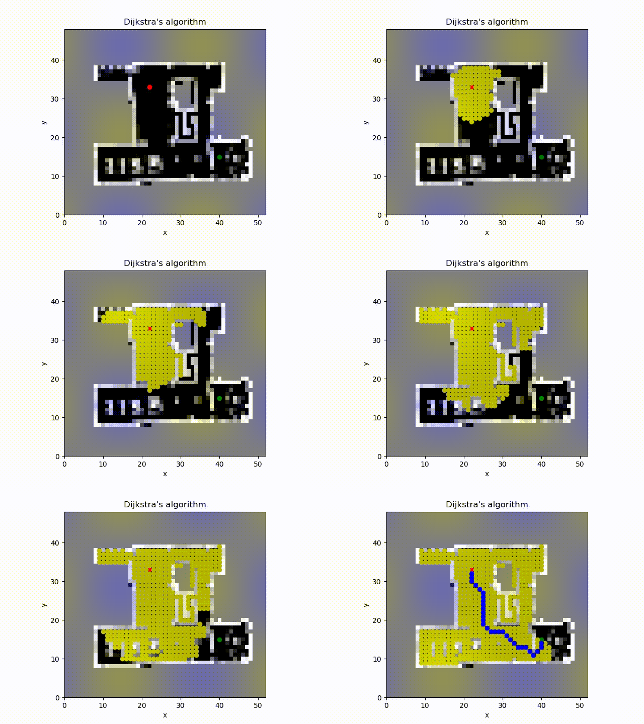
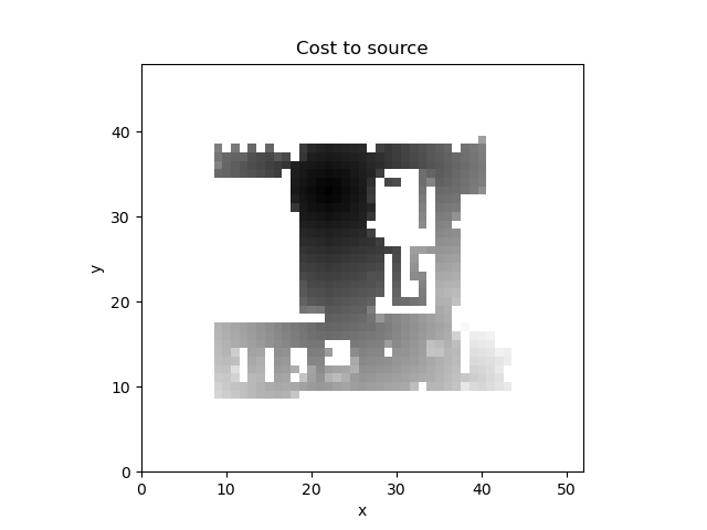
Dijkstra’s algorithm finds the optimal solution, i.e., the path with the least path cost.

A* algorithm with constant factor 1 also finds the optimal solution but with fewer number of cell expanded.

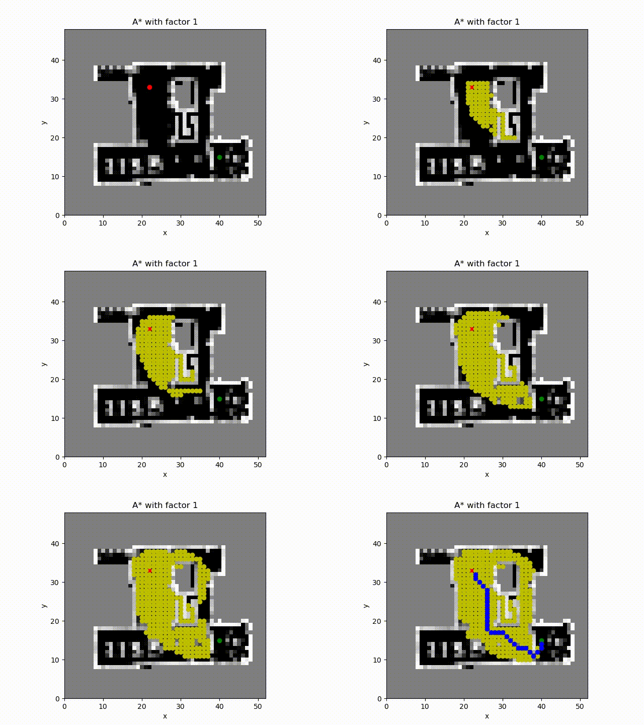
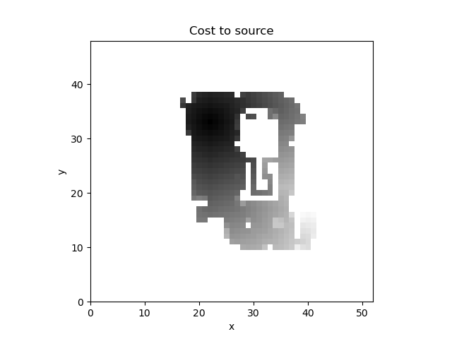
A* algorithm with constant factor 2 which inflates the estimate of the cost to the goal from the cell. The number of cell expanded is much more smaller and the path cost is close to the optimal path.

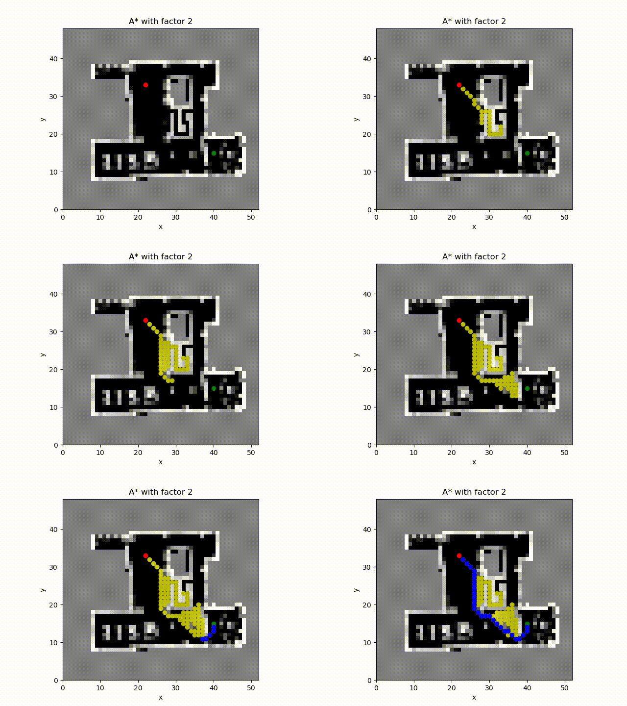
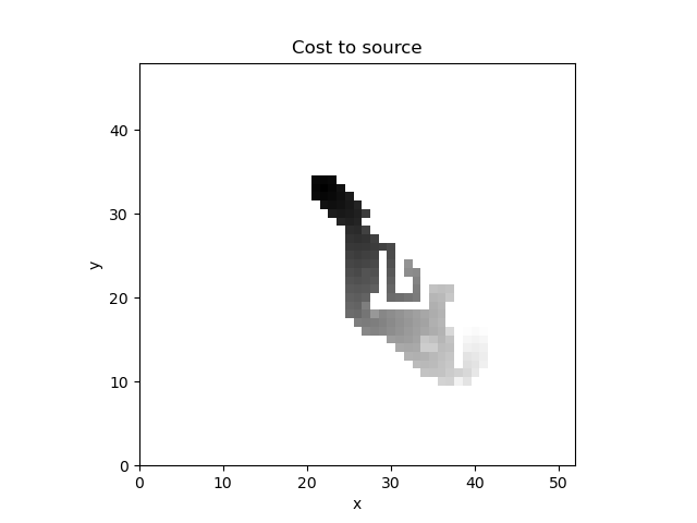
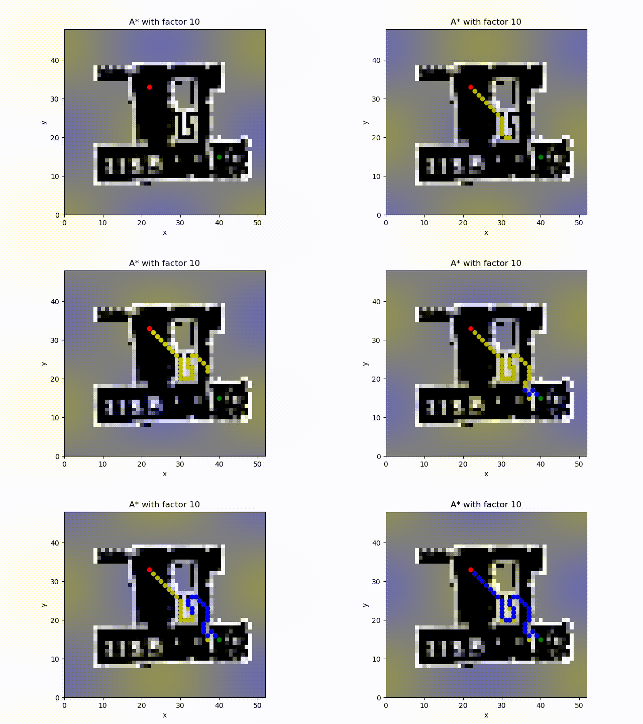
A* algorithm with constant factor 5. The obtained path length is smaller than others. The reason is that when computing the tentative cost the path length has higher weight than the path cost which includes the occupancy probability.

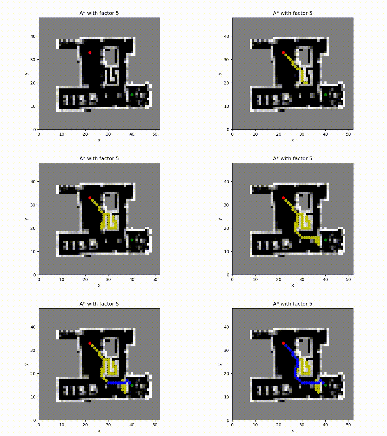
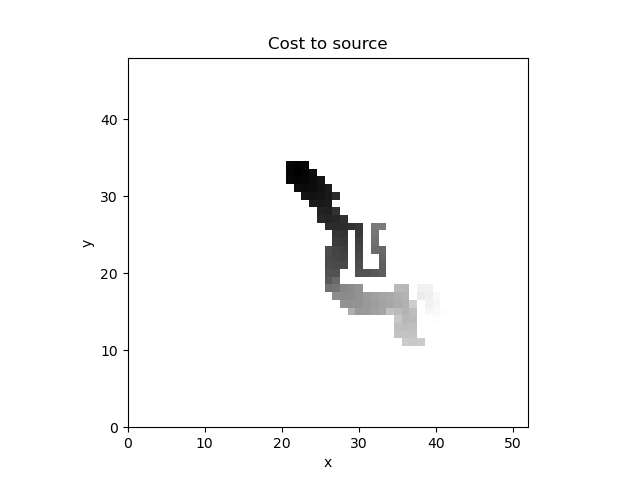
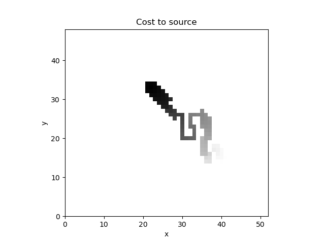
A* algorithm with constant factor 10. Even though the constant factor is larger, the path path does not reduce accordingly. The reason could be that the heuristic is not admissible if we consider only the path length. In other words the heuristic value is greater than the optimal path length.